Can
Bias Mask Primordial Non-Gaussianity?
David Weinberg (advisor)
: Bryan Gymrek : Susan Kassin
: Aaron Sokasian
(based
on Non-Gaussian
Fluctuations and the Statistics of Galaxy Clustering
by Weinberg and Cole)
I.
Introduction
II. Biasing Scheme
III. Statistics and Conclusions
I.
Introduction
The Large Scale Structure that we observe today is believed to have grown
from small amplitude fluctuations made by physical processes in the early
universe. Gravitational instability amplifies these fluctuations;
they form the clusters, walls, and filaments that we observe today.
The usual assumption is that the initial fluctuations were a Gaussian random
field. We explore the possibility of a non- Gaussian initial field.
If a non-Gaussian field is evolved forward in time to z=0, it will not
produce the Gaussianness of the mass distribution that we see today.
However, if we include a particular biasing scheme, can we produce the
large scale structure that's observed today? We try to answer this
question with a cosmological n-body code.
A.
Evolution of Structure
These
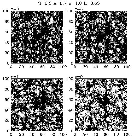
are examples of Cartesian slices through our particle distribution (1/20
th. of a 100 h-1 Mpc cube):
Gaussian
initial conditions are used, and no biasing scheme is implemented.
We use a CDM power spectrum and normalize the amplitude to the parameter
sigma-8, the rms fluctuations of galaxy counts in 8 h-1 Mpc spheres.

The eye is effective at noticing patterns and subtle qualities. One
can reject models based on appearance alone; however, they must keep in
mind observational procedures if they are comparing them to observational
data. Here, we concentrate on comparing models to each other.
B.
Non-Gaussian Initial Fluctuations
1.
Why might we need them?
One example of a physical process in the early universe that could have
produced non-Gaussian initial fluctuations comes from the multiple field
inflationary model. In this theory, quantum fluctuations of an inflation
scalar field provide the underlying Gaussian random field, as usual.
However, there also exists a second scalar field, energetically unimportant
during inflation, but responsible for producing baryons and axions.
If this field depended on the inflationary field through a non-linear function,
then Gaussian quantum fluctuations in the inflationary field would induce
non-Gaussian fluctuations in the secondary field. This would lead
to non-Gaussian fluctuations in the matter density.
2.
What are they?
Primordial density fluctuations form a Gaussian random field if the field's
Fourier components delta(k) have independent, random phases.
density field = delta(x)
= sum of delta(k) * e -2 pi ikx
delta(k) = Ak
ei*thetak
where
thetak are the phases. The power spectrum can therefore
be written,
P(k) = <Re
2delta(k)> + <Im
2 delta(k)>.
Therefore,
the random phase condition guarantees that the one-point probability distribution,
P(x) is Gaussian.
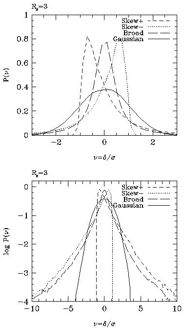
Non-Gaussian models are characterized by their one-point probability functions.
Models with a long tail of positive fluctuations are called "skew positive;"
those with a long negative tail are "skew negative." And, those with
tails of both the skew positive and the skew negative distributions are
called "broad."

The
skew positive models are motivated by theories of global texture and global
monopoles. They form structure by accreting
mass onto high peaks of the density field, leaving large voids unperturbed.
This leaves a lumpy, voidless structure.
Skew
negative scenarios rely on motivation from the "explosion model," where
negative density fluctuations behave like gravitational explosions that
sweep matter out of low density areas. These models possess minima
that develop into expanding bubbles.
Broad
models share the characteristics of both the skew positive and skew negative
models.
Here
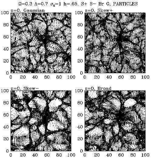
are slices of our simulation at z=0 for different initial conditions:

Notice
how filaments, clusters, low density regions form at similar locations
in all four simulations. This is because all four sets of initial
conditions are generated by approximately monotonic transformations, M,
of the same underlying field. Each model has distinctive structure
because of the probability distribution of initial conditions.
3.
How do we produce non-Gaussian initial conditions?
We start with a Gaussian random field that contains a CDM power spectrum.
Next, we smooth this field with a Gaussian filter of 3 Mpc, the scale where
the rms fluctuations are just going non-linear today. We then make
a monotonic, local transformation, M, to get to the non-Gaussain field.
The transformation stretches and/or compresses the features of the smoothed
Gaussian random field. It turns it into a field that has a skew positive,
skew negative, or broad probability distribution function. (By an
appropriate choice of transformation, one can distort the probability distribution
function into an arbitrary form.) Finally, we un-smooth the field.
This inverts the Gaussian filter and restores the original power spectrum.
F = Gaussian random field,
P(F) = (-1 / sqrt (2 pi) ) e-(F^2)/2
|
|
v
smooth with Gaussian filter
|
|
v
monotonic, local transformation, M
to get to non-Gaussian field
D = distorted non-Gaussian random field
D(r) = M [ F(r) ],
P(D) = P(F) |dM/dF|-1
|
|
v
unsmooth: invert Gaussian filter
and restore original power spectrum
3.
Biasing
A particular global biasing scheme determines how luminous matter follows
the dark matter distribution calculated in the simulation. If gravity
was a linear force, and we added a generic bias scheme, then a system with
non-linear initial conditions would evolve linearly to match the Gaussianness
observed today. However, since gravity is a non-linear force, the
system with non-linear initial conditions evolves non-linearly into structure
that doesn't match the Gaussianity of today. (Keep in mind that a
model with Gaussian initial conditions would evolve non-linearly to match
the structure of today.)
Linear:
Gaussian model--> Non-Gaussian model + Bias
--evolve--> match
Gaussian observations today
Non-linear:
Gaussian model--> Non-Gaussian model + Bias
-^-non-linear evolve-^->
doesn't match
(gravity)
Gaussian model + Bias
-^-non-linear evolve-^->
match
The goal of our project is to test if non-Gaussian initial conditions,
coupled with a particular biasing scheme, are able to produce the same
Gaussian structure that a model with Gaussian initial conditions produces
at z=0. We used a biasing algorithm, "match bias," that tried
to match the one-point probability distribution functions of the Gaussian
and non-Gaussian fields.
Non-linear:
Gaussian model-->
Non-Gaussian model + MATCH BIAS -^->
match?
more
on biasing...
Back to Computing Our Universe 1999
-<Susan Kassin>
