The theory behind this interaction has been discussed in depth in the sources cited on our References page. We will therefore give a quantitative approach here and direct the interested reader to the sources listed there. The satellite galaxy will often be referred to as "the perturber."
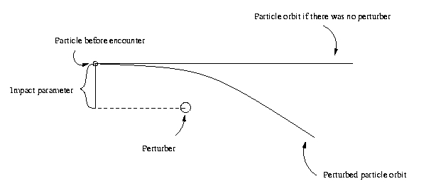
The first stage of understanding dynamical friction is understanding what happens to the orbit of a particle (let's call it particle 1) when it passes another particle (let's call it particle 2). Suppose that particle 2 is at rest in the frame where we study the encounter. The orbit of particle 1 will look like this:
The next step is to understand what happens when a point mass (the perturber) moves through system of particles. One can study (Binney and Tremaine) the cumulative effect of all the encounters. In the case where the orbits of the particles in the system is solely determined by their initial distribution function and the gravitational force from the perturber, one can show that there is no overall change in velocities in the direction perpendicular to that of the perturber's velocity. However, there is a change in velocity parallel to the direction of travel of the perturber. One can further show that these changes in velocities results in an overdensity of particles behind the perturber. The cumulative gravitational attraction from this overdensity will slow the perturber down. This effect is called dynamical friction. The overdensity behind the perturber is called a wake.
We're not really interested in the way that the system slows down the perturber but in the way that the perturber changes the general properties of the system. Since the perturber disturbs the orbits of the particles in the system, it introduces a density perturbation that disturbs the equilibrium of the system. We're interested in the properties of the density perturbation and the evolution of this density perturbation with time. The parameters that characterize the perturbation are:
Our simulation was carried out with an N-body code created by our advisor, Martin Weinberg. The code is based on a biorthogonal expansion method; it represents the system as a truncated series of expansion functions. This code has the advantage of being very fast (it scales as order N, which is great as N-body codes go) but is limited to simulations in which the system does not diverge greatly from a spherically symmetric distribution.
The code uses a system of dimensionless units such that 1 unit of length corresponds to 7 kpc, 1 unit of mass is 1011 Msun (the luminous mass of the Milky Way), and 1 unit of time corresponds to 0.095 galactic year (at the solar circle). From this point on, all references to measurements will be made in these units.
We ran a total of three simulations, in each case the mass of the perturber was 0.3 and the mass of the halo was 10 (the halo is 10 times as massive as the luminous matter). The perturber followed a straight trajectory parallel to the z-axis with an impact parameter b = 2.3 along the x-axis. The halo was composed of 200,000 particles, a number chosen as a compromise between speed and resolution. Below is a view of the initial and final conditions of our simulation in which v = 1.0.
 |
 |
The first simulation had a velocity of 1.0, the second 2.0, and the third 0.5. We chose to vary velocity for a number of reasons. Among these, the most important was the effect of velocity on the amplitude and longevity of the wake. Choosing to vary velocity also simplified the situation somewhat. Had we chosen to vary impact parameter, the gravitational interaction between the satellite and the halo would have become significant.
The simulations were set up to run for 100 time units, with a time step of 0.01 units. The code was set up such that at t = 50 the perturber would cross the x-y plane, making its closest approach to the center of the halo.
We needed to locate the perturber and mark its position every time we created an image in TIPSY. This was easily done given the velocity and the time with respect to t = 50.
The N-body code produced a variety of data about the particles at predetermined intervals. With the use of another program we were able to generate TIPSY arrays, which we could then plot along with the actual positions to generate many of the plots shown in the Results section. Among the data generated were density, relative density, velocities, potential energies, and relative potential energies. These data were very useful in finding the wake, which is a very weak effect. For more on how this was done, see the Analysis & Interpretation section on the Results page.