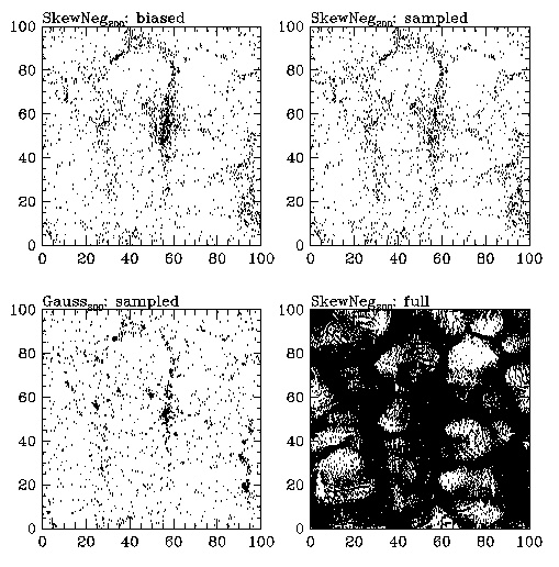
SKEW NEGATIVE:
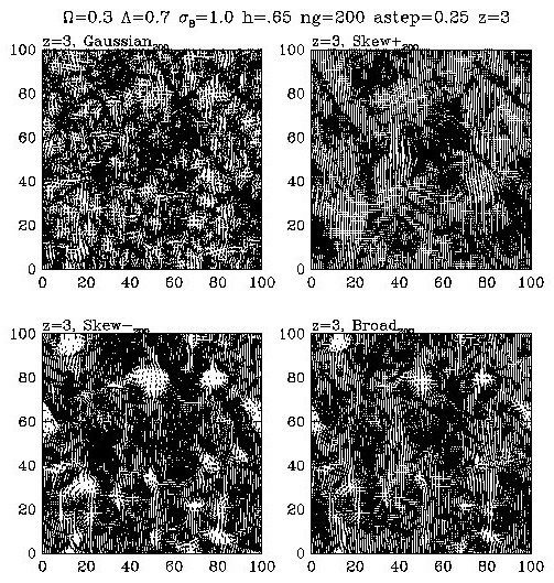
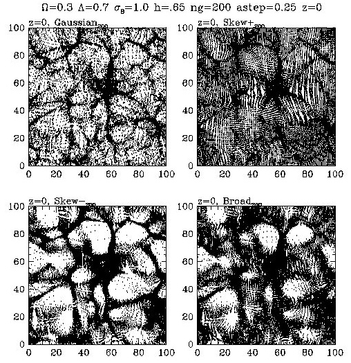
As you can see, none of
the other models really succeds in mimicking
the Gaussian plot, which
is what we want. Mabye the Skew+ looks
relatively similar to
the Gaussian (in the z=0 plot), but the lack of underdense
regions in the S+ plot
is an obvious flaw.
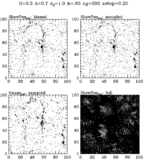
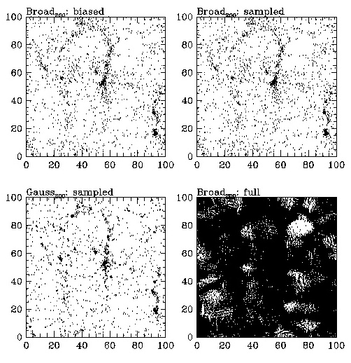
Here are three more particle
plots that show the biased, sampled version of
the model in the upper
left, the sampled in the upper right, the Gaussian
sampled in the lower
left, and the full version of the model in the lower
right.
Please compare by eye
the upper left (biased S+, S-, or Broad) to the lower
left (the sampled Gaussian).
If our biasing sheme were really masking
primordial non-Gaussianity,
then the two plots on the left would be
identical. However,
as you can check for yourself, they are different.
This is our first piece
of evidence that biasing is NOT masking the primordial
non-Gaussianity.
SKEW POSITIVE:
SKEW NEGATIVE:
BROAD:
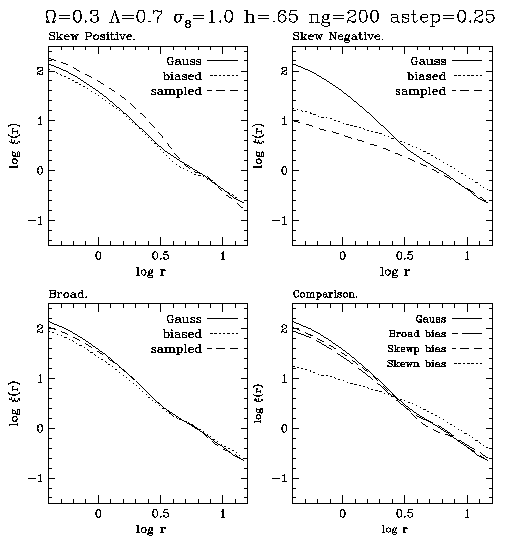
First, we look at the
correlation function. The correlation
function is
defind in the Weinberg
and Cole paper as:
"If you start from a randomly
chosen galaxy, this (the correlation function)
gives the excess probability
of finding a second galaxy at a distance r."
In simpler terms, it is
a measure of the density as a function of r.
Here is the correlation
function graph for the three models, with
the lower right graph
containg all three plus the gaussian plotted
together.
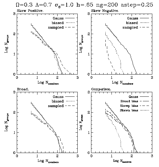
Next, we examine the group multiplicity
function. This statistic is simpler
than it sounds. Basically,
we assign galaxies to groups using a friends
of friends algroithm (which
uses a linking length of .2 times the mean
interparticle separation.)
This basically makes clusters of galaxies. Then
we plot the # of groups vs.
the # of members in the group. In this way
we can see how many galaxy clusters
there are as a function of the number
of members in the cluster.
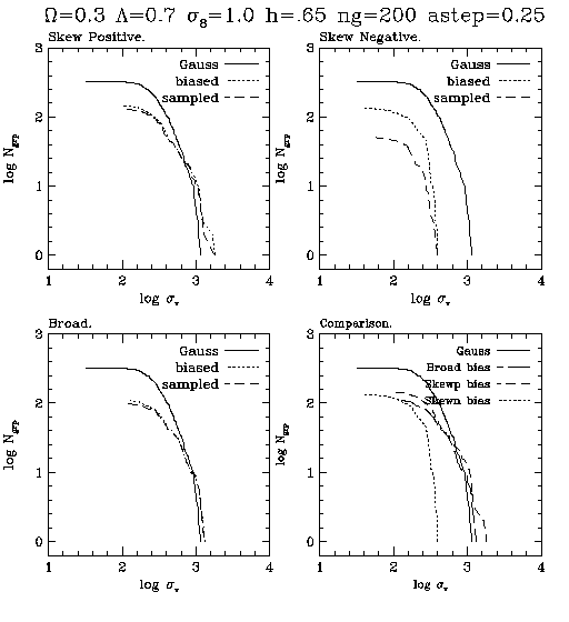
Another important statistic is the cumulative
"temperature funciton"
This is important because it
can be used to extimate the potential depth, or
"virial temperature" and is
measured observationally. We plot here:
log Ngroups (>Sigmav)
vs Sigmav . This is the number density of groups
with 1D velocity dispersion
greater than Sigmav .
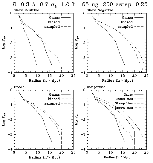
The last statistic that we will examine is the underdense
probability funciton.
This one is a little confusing
at first, but it is just basically a measure
of the underdensity as a function
of radius. the strict definition is that the UPF
is the "Probability that the
average density in a randomly placed sphere
of radius r is more than 80%
below the mean density." Just remember that
it is basically a measure of
the underdensity on different scales.
Since Gaussian initial fluctiuations
fit the observed data far better
than any of the other models
(even when they are biased) there
is no reason to believe that
the S+, S-, or Broad models could
have produced the large scale
structure that we see today.
Back to main project page